Introduction
In this study, two different methods to calculate steady-state probability distribution of randomly created transition probability matrices will be investigated, along with the effect of the inclusion of absorbing states. One can reach the R Markdown file used to create this report from the GitHub repository of the exercise.
Library Imports and Parameter Definitions
The only extra-Base-R library that will be included in this work is ggplot2, which will be used to generate comparison plots.
1
2
3
4
5
6
7
8
9
| # Library imports
library(ggplot2)
# Defining the parameters
seed <- 203
M <- 200000
E <- 0.0005
|
Generating Transition Probability Matrices
To generate transition probability matrices in a practical way, a function that takes the matrix size as an argument can be defined as follows:
1
2
3
4
5
6
7
8
9
10
11
12
13
14
15
16
17
18
19
20
21
22
23
24
25
26
| GenerateTPM <- function(n) { # Creating a function that generates
# transition probability matrices
TPM <- matrix( , # Creating an empty (n+1) x (n+1) matrix
nrow = n+1,
ncol = n+1)
for (i in 1:(n+1)) { # Filling the matrix with random numbers
# between 0 and 1
for (j in 1:(n+1)) {
TPM[i,j] <- runif(1) # Random numbers from uniform distribution
}
}
for (i in 1:(n+1)) { # Adjusting the matrix such that
# all the rows sum up to 1
TPM[i,] <- TPM[i,]/sum(TPM[i,])
}
return(TPM)
}
|
The next step is to create 3 different transition matrices:
- P1 with n=5,
- P2 with n=25,
- P3 with n=50
1
2
3
4
5
6
7
8
9
| set.seed(seed)
P1 <- GenerateTPM(5)
P2 <- GenerateTPM(25)
P3 <- GenerateTPM(50)
# The appearance of the smallest matrix can be checked to keep track
print(round(P1, 2))
|
1
2
3
4
5
6
7
| ## [,1] [,2] [,3] [,4] [,5] [,6]
## [1,] 0.09 0.24 0.24 0.09 0.21 0.13
## [2,] 0.25 0.36 0.04 0.00 0.17 0.19
## [3,] 0.25 0.25 0.06 0.17 0.23 0.05
## [4,] 0.08 0.00 0.15 0.13 0.37 0.27
## [5,] 0.06 0.09 0.10 0.30 0.16 0.29
## [6,] 0.16 0.15 0.26 0.15 0.26 0.02
|
Applying Monte Carlo Simulation
To apply Monte Carlo Simulation with the created matrices, a function that takes one matrix and one number for repetitions as arguments can be defined:
1
2
3
4
5
6
7
8
9
10
11
12
13
14
15
16
17
18
19
20
21
22
23
24
25
26
27
28
29
30
31
32
33
34
35
36
37
38
39
40
41
42
| MonteCarlo <- function(TPM, n) {
size <- nrow(TPM) # Creating a variable to store
# the size of the matrix
X0 <- sample(1:size, 1) # Setting the initial state
activeState <- X0 # Initializing the variable that
# stores the current state
statesVec <- c() # Creating a vector to keep track of
# the occurrence of states
for (rep in 1:n) { # Creating a loop to control
# the switches between states
r <- runif(1) # Assigning the random value of "r"
cdf <- c(0, cumsum(TPM[activeState, ]))
for (j in 1:size) { # Creating a loop to determine
# the interval of "r",
# and also to update the current state
# and the occurrence sequence accordingly
if ((r > cdf[j] ) &&
(r <= cdf[j+1]) ) {
activeState <- j
statesVec <- append(statesVec, j)
}
}
}
return(table(statesVec)/n)
}
|
Simulating with the previously obtained probability matrices yields the following steady-state distributions:
1
2
3
4
5
6
7
8
9
10
11
12
13
14
15
| exeTimes <- data.frame(row.names = c("Monte Carlo", # Creating an empty data frame
"Matrix Mult."), # to store execution times
P1 = numeric(2),
P2 = numeric(2),
P3 = numeric(2) )
set.seed(seed)
exeTimes[c("Monte Carlo"), c("P1")] <- Sys.time()
P1MC <- MonteCarlo(P1, M)
exeTimes[c("Monte Carlo"), c("P1")] <- Sys.time() - exeTimes[c("Monte Carlo"), c("P1")]
P1MC
|
1
2
3
| ## statesVec
## 1 2 3 4 5 6
## 0.143100 0.177635 0.136880 0.148900 0.225485 0.168000
|
1
2
3
4
5
6
7
| exeTimes[c("Monte Carlo"), c("P2")] <- Sys.time()
P2MC <- MonteCarlo(P2, M)
exeTimes[c("Monte Carlo"), c("P2")] <- Sys.time() - exeTimes[c("Monte Carlo"), c("P2")]
P2MC
|
1
2
3
4
5
6
7
8
9
| ## statesVec
## 1 2 3 4 5 6 7 8
## 0.043520 0.032165 0.043510 0.042040 0.043160 0.036385 0.037285 0.041145
## 9 10 11 12 13 14 15 16
## 0.042865 0.039145 0.040090 0.035130 0.037885 0.033085 0.035305 0.035915
## 17 18 19 20 21 22 23 24
## 0.032975 0.031045 0.037090 0.043020 0.043805 0.033115 0.039085 0.039055
## 25 26
## 0.043275 0.038905
|
1
2
3
4
5
6
7
| exeTimes[c("Monte Carlo"), c("P3")] <- Sys.time()
P3MC <- MonteCarlo(P3, M)
exeTimes[c("Monte Carlo"), c("P3")] <- Sys.time() - exeTimes[c("Monte Carlo"), c("P3")]
P3MC
|
1
2
3
4
5
6
7
8
9
10
11
12
13
14
15
| ## statesVec
## 1 2 3 4 5 6 7 8
## 0.021075 0.018225 0.019560 0.019240 0.018770 0.020910 0.017380 0.017940
## 9 10 11 12 13 14 15 16
## 0.019640 0.019665 0.022670 0.020470 0.020085 0.019405 0.017140 0.018220
## 17 18 19 20 21 22 23 24
## 0.019765 0.020750 0.015515 0.018245 0.018785 0.017710 0.022470 0.017800
## 25 26 27 28 29 30 31 32
## 0.021980 0.019665 0.018545 0.021540 0.021550 0.020760 0.017310 0.018465
## 33 34 35 36 37 38 39 40
## 0.020820 0.020365 0.018765 0.020685 0.022740 0.023395 0.018875 0.016125
## 41 42 43 44 45 46 47 48
## 0.018185 0.019380 0.020755 0.018655 0.020260 0.020795 0.019210 0.021725
## 49 50 51
## 0.018700 0.017200 0.022115
|
Applying Martix Multiplication Method
A function that takes P and a stopping condition parameter ε and applies matrix multiplication until the length of the difference between a randomly selected row and row averages is less than ε can be defined as follows:
1
2
3
4
5
6
7
8
9
10
11
12
13
14
15
16
17
18
19
20
21
22
23
24
25
26
27
28
29
30
31
| matrixMult <- function(TPM, E) {
activeMatrix <- TPM
piBar <- colMeans(activeMatrix) # Average of rows
# stored in a vector
randomRow <- sample(1:nrow(activeMatrix), 1) # Picking a random row
convergence <- sqrt(sum( # A logical variable that
(activeMatrix[randomRow, ] - piBar )^2) ) < E # indicates whether
# the current convergence
# is sufficient
while (!convergence) { # Updating the local variables
# until the convergence condition
# is satisfied
activeMatrix <- activeMatrix %*% activeMatrix # Matrix multiplication
piBar <- colMeans(activeMatrix)
randomRow <- sample(1:nrow(activeMatrix), 1)
convergence <- sqrt(sum((activeMatrix[randomRow, ] - piBar)^2)) < E
}
return(piBar)
}
|
1
2
3
4
5
6
7
8
9
| set.seed(seed)
exeTimes[c("Matrix Mult."), c("P1")] <- Sys.time()
P1MM <- matrixMult(P1, E)
exeTimes[c("Matrix Mult."), c("P1")] <- Sys.time() - exeTimes[c("Matrix Mult."), c("P1")]
P1MM
|
1
| ## [1] 0.1418896 0.1752635 0.1367005 0.1508137 0.2276087 0.1677241
|
1
2
3
4
5
6
7
| exeTimes[c("Matrix Mult."), c("P2")] <- Sys.time()
P2MM <- matrixMult(P2, E)
exeTimes[c("Matrix Mult."), c("P2")] <- Sys.time() - exeTimes[c("Matrix Mult."), c("P2")]
P2MM
|
1
2
3
4
5
| ## [1] 0.04261998 0.03275381 0.04323659 0.04276693 0.04295757 0.03671693
## [7] 0.03694794 0.04117294 0.04242615 0.03842398 0.04019447 0.03560988
## [13] 0.03771862 0.03295448 0.03598425 0.03575689 0.03313544 0.03162181
## [19] 0.03708412 0.04285083 0.04333381 0.03306816 0.03928567 0.03890044
## [25] 0.04354170 0.03893662
|
1
2
3
4
5
6
7
| exeTimes[c("Matrix Mult."), c("P3")] <- Sys.time()
P3MM <- matrixMult(P3, E)
exeTimes[c("Matrix Mult."), c("P3")] <- Sys.time() - exeTimes[c("Matrix Mult."), c("P3")]
P3MM
|
1
2
3
4
5
6
7
8
9
| ## [1] 0.02036234 0.01811745 0.01958708 0.01933626 0.01850812 0.02098865
## [7] 0.01734776 0.01838142 0.01958771 0.01913874 0.02268059 0.02094601
## [13] 0.01978689 0.01907543 0.01730207 0.01811857 0.01923823 0.02069250
## [19] 0.01549397 0.01832879 0.01855905 0.01765549 0.02279090 0.01745068
## [25] 0.02238944 0.01951077 0.01893984 0.02127761 0.02170173 0.02076694
## [31] 0.01758487 0.01852527 0.02110391 0.01969839 0.01914967 0.01991998
## [37] 0.02259353 0.02353297 0.01934586 0.01617337 0.01900646 0.01907645
## [43] 0.02077114 0.01867158 0.02087822 0.02070635 0.01963375 0.02154106
## [49] 0.01849888 0.01731532 0.02221192
|
Comparison of the Results Obtained by Two Different Methods
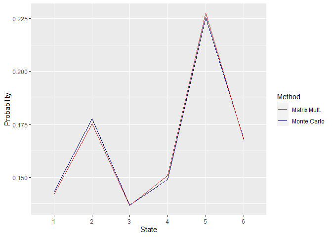
First off, the similarity between the obtained steady-state distributions by the two methods can be checked. This can be done by plotting the distributions.
1
2
3
4
5
6
7
8
9
10
11
12
13
14
15
16
17
| ggplot(data.frame(P1MC, P1MM),
aes(x = statesVec) ) +
geom_line(aes(y = Freq,
color = 'Monte Carlo',
group = 1) ) +
geom_line(aes(y = P1MM,
color = 'Matrix Mult.',
group = 1) ) +
labs(x = "State",
y = "Probability") +
scale_color_manual(name = "Method",
values = c("Monte Carlo" = "darkblue",
"Matrix Mult." = "firebrick3") )
|
Figure 1. Steady State Distributions Obtained Using P1
1
2
3
4
5
6
7
8
9
10
11
12
13
14
15
16
17
| ggplot(data.frame(P2MC, P2MM),
aes(x = statesVec) ) +
geom_line(aes(y = Freq,
color = 'Monte Carlo',
group = 1) ) +
geom_line(aes(y = P2MM,
color = 'Matrix Mult.',
group = 1) ) +
labs(x = "State",
y = "Probability") +
scale_color_manual(name = "Method",
values = c("Monte Carlo" = "darkblue",
"Matrix Mult." = "firebrick3") )
|
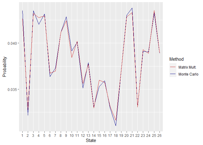
Figure 2. Steady State Distributions Obtained Using P2
1
2
3
4
5
6
7
8
9
10
11
12
13
14
15
16
17
18
19
| ggplot(data.frame(P3MC, P3MM),
aes(x = statesVec) ) +
geom_line(aes(y = Freq,
color = 'Monte Carlo',
group = 1) ) +
geom_line(aes(y = P3MM,
color = 'Matrix Mult.',
group = 1) ) +
labs(x = "State",
y = "Probability") +
theme(axis.text.x = element_blank()) +
scale_color_manual(name = "Method",
values = c("Monte Carlo" = "darkblue",
"Matrix Mult." = "firebrick3") )
|
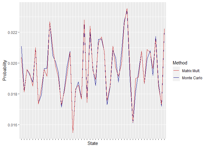
Figure 3. Steady State Distributions Obtained Using P3
As can be seen in the above plots, the distributions are quite close, and their difference increases when the size of the matrix P is increased. This can be associated with the fact that higher matrix sizes retard convergence.
Next, execution times can be checked as follows:
1
| print(round(exeTimes, 3))
|
1
2
3
| ## P1 P2 P3
## Monte Carlo 35.479 37.226 37.697
## Matrix Mult. 0.319 0.002 0.000
|
There is a huge difference between the run times, probably due to the large M value used during Monte Carlo Simulations. Keeping in the mind that the two methods have given similar distributions, it can be concluded that matrix multiplication method works more efficiently. This stems from its exponential-like approach, being multiplying the matrix P by itself repeatedly, that allows the algorithm to skip unnecessary calculations, while Monte Carlo Simulation calculates each state one by one.
Checking the Case with Absorbing States
To include an absorbing state, one element in the diagonal should be set to 1, in other words, in each matrix there should be one element that satisfies the condition pjj. Simply, p11, p22, p33 can be selected for P1, P2, P3, respectively:
1
2
3
4
5
6
7
8
| P1Abs <- P1
P2Abs <- P2
P3Abs <- P3
P1Abs[2, ] <- c(0, 1, rep(0, 4)) # Row number is 1+1, since R starts indexing
# from 1 instead of 0
P2Abs[3, ] <- c(0, 0, 1, rep(0, 23))
P3Abs[4, ] <- c(0, 0, 0, 1, rep(0, 47))
|
1
2
3
4
5
6
7
8
9
10
11
12
13
14
15
16
| exeTimesAbs <- data.frame(row.names = c("Monte Carlo", # Creating an empty data frame
"Matrix Mult."), # to store execution times
P1 = numeric(2),
P2 = numeric(2),
P3 = numeric(2) )
set.seed(seed)
exeTimesAbs[c("Monte Carlo"), c("P1")] <- Sys.time()
P1AbsMC <- MonteCarlo(P1Abs, M)
exeTimesAbs[c("Monte Carlo"), c("P1")] <- Sys.time() -
exeTimesAbs[c("Monte Carlo"), c("P1")]
P1AbsMC
|
1
2
3
| ## statesVec
## 2 3
## 0.999995 0.000005
|
1
2
3
4
5
6
7
8
| exeTimesAbs[c("Monte Carlo"), c("P2")] <- Sys.time()
P2AbsMC <- MonteCarlo(P2Abs, M)
exeTimesAbs[c("Monte Carlo"), c("P2")] <- Sys.time() -
exeTimesAbs[c("Monte Carlo"), c("P2")]
P2AbsMC
|
1
2
3
4
5
| ## statesVec
## 3 4 5 7 13 15 19 20
## 0.999945 0.000015 0.000005 0.000005 0.000005 0.000005 0.000005 0.000005
## 21 24
## 0.000005 0.000005
|
1
2
3
4
5
6
7
8
| exeTimesAbs[c("Monte Carlo"), c("P3")] <- Sys.time()
P3AbsMC <- MonteCarlo(P3Abs, M)
exeTimesAbs[c("Monte Carlo"), c("P3")] <- Sys.time() -
exeTimesAbs[c("Monte Carlo"), c("P3")]
P3AbsMC
|
1
2
3
4
5
| ## statesVec
## 2 3 4 8 13 14 19 22
## 0.000005 0.000005 0.999945 0.000005 0.000005 0.000005 0.000005 0.000005
## 25 28 46
## 0.000005 0.000010 0.000005
|
1
2
3
4
5
6
7
8
9
10
| set.seed(seed)
exeTimesAbs[c("Matrix Mult."), c("P1")] <- Sys.time()
P1AbsMM <- matrixMult(P1Abs, E)
exeTimesAbs[c("Matrix Mult."), c("P1")] <- Sys.time() -
exeTimesAbs[c("Matrix Mult."), c("P1")]
P1AbsMM
|
1
2
| ## [1] 1.515655e-05 9.998906e-01 1.915830e-05 2.327182e-05 3.069990e-05
## [6] 2.114914e-05
|
1
2
3
4
5
6
7
8
| exeTimesAbs[c("Matrix Mult."), c("P2")] <- Sys.time()
P2AbsMM <- matrixMult(P2Abs, E)
exeTimesAbs[c("Matrix Mult."), c("P2")] <- Sys.time() -
exeTimesAbs[c("Matrix Mult."), c("P2")]
P2AbsMM
|
1
2
3
4
5
6
| ## [1] 1.217847e-04 8.934742e-05 9.973187e-01 1.240207e-04 1.247643e-04
## [6] 9.977755e-05 1.020275e-04 1.137461e-04 1.237126e-04 1.051454e-04
## [11] 1.147747e-04 9.908271e-05 1.032044e-04 9.266297e-05 1.041990e-04
## [16] 9.780057e-05 9.190099e-05 9.137568e-05 1.011092e-04 1.187355e-04
## [21] 1.193959e-04 9.426228e-05 1.076331e-04 1.127492e-04 1.195337e-04
## [26] 1.085060e-04
|
1
2
3
4
5
6
7
8
| exeTimesAbs[c("Matrix Mult."), c("P3")] <- Sys.time()
P3AbsMM <- matrixMult(P3Abs, E)
exeTimesAbs[c("Matrix Mult."), c("P3")] <- Sys.time() -
exeTimesAbs[c("Matrix Mult."), c("P3")]
P3AbsMM
|
1
2
3
4
5
6
7
8
9
| ## [1] 0.001635044 0.001455174 0.001568544 0.920604415 0.001470199 0.001687420
## [7] 0.001399524 0.001473365 0.001575034 0.001523901 0.001823980 0.001690725
## [13] 0.001613915 0.001560759 0.001419325 0.001487944 0.001558805 0.001663124
## [19] 0.001269764 0.001484766 0.001519511 0.001435973 0.001831733 0.001385525
## [25] 0.001814823 0.001593939 0.001548640 0.001719198 0.001767902 0.001705231
## [31] 0.001439168 0.001518595 0.001686385 0.001594235 0.001561261 0.001599391
## [37] 0.001819802 0.001920896 0.001555786 0.001276327 0.001562249 0.001563628
## [43] 0.001715398 0.001498189 0.001685407 0.001660050 0.001598088 0.001771775
## [49] 0.001478922 0.001408776 0.001797467
|
As can be expected, in both methods, absorbing states have the major part of the total probability, reducing the other states to negligible steady-state probabilities. In all of the cases, their steady-state probabilities are above 90%, due to the infinite loop that starts after the first encounter with the absorbing state.
An important difference between the two methods this time is that Monte Carlo Simulation has 0 probabilities for some states in all three simulations, while the matrix multiplication method yields a steady-state distribution consisting full of non-zero values. This is because Monte Carlo Simulation is a more practical method and it only assigns non-zero probabilities to the states that occur before the first occurrence of the absorbing state during the simulation process. On the other side, the matrix multiplication method works in a theoretical way and assigns a small probability to every non-absorbing state.
When it comes to execution times, the new results are as follows:
1
| print(round(exeTimesAbs, 3))
|
1
2
3
| ## P1 P2 P3
## Monte Carlo 44.896 37.699 37.463
## Matrix Mult. 0.001 0.003 0.003
|
It would not be fair to draw any conclusions from the execution times since there is no significant change or any obvious behaviors in differences between the trials with and without absorbing states. However, with a more elaborate work, the above algorithm implemented for Monte Carlo Simulation can be enhanced by the addition of some extra rules that stop iterations after the first occurrence of the absorbing state since from that point on there will be no change of state, and this would potentially reduce the execution time dramatically by eliminating redundant calculations.
IE 203 - Operations Research II
Boğaziçi University - Industrial Engineering Department
GitHub Repository