Introduction
In this study, the effects of parameters and neighborhood functions on the results of Self-Organizing Maps solution for Traveling Salesman Problem will be investigated.
The algorithms have been run on the data set that includes the coordinates of Turkish provinces. The seventh trial (M = 3n, 100 iterations) yields the optimal solution for TSP with Turkish provinces.
Do not forget to check the GitHub repository!
The first step is to import libraries and data, along with setting the seed for consistent results.
1
2
3
4
5
6
7
8
9
10
11
12
13
14
# Required libraries for plots

library(ggplot2)
library(dplyr)
library(ggrepel)
library(tidyr)

data <- read.table("Data.txt",
                   header = TRUE,           # Data includes column names
                   encoding = "UTF-8")      # For Turkish characters

seed <- 440

set.seed(seed)
Function Definitions
1
2
3
4
5
6
7
8
9
10
11
12
13
14
15
16
17
18
19
20
21
22
23
24
25
26
27
28
29
30
31
32
33
34
35
36
37
38
39
40
41
42
43
44
45
46
47
48
49
50
51
52
53
54
55
56
57
58
59
60
61
62
63
64
65
66
67
68
69
70
71
72
73
74
75
76
77
78
79
80
81
82
83
84
85
86
87
88
89
90
# Functions to calculate Euclidean Norm and Euclidean Distance

enorm <- function(x, y) sqrt(x^2 + y^2)
edist <- function(vect1, vect2) sqrt(sum((vect1 - vect2)^2))

# Neighborhood function 1: Gaussian Kernel

gaussian_kernel <- function(I, w, sigma, ip, i){

    h <- exp(-edist(w[i, ], w[ip, ])^2 / (sigma^2))

    return(h)
}

# Neighborhood function 2: Elastic Band

elastic_band <- function(I, w, sigma, ip, i){

    d <- min(abs(i-ip), I-abs(i-ip))
    A <- exp(-(d^2)/(sigma^2))

    return(A)
}

# A function to convert algorithm outputs to travel plans
# (Will only be used inside the function "results")

route <- function(X, w){    # X: cities, w: neurons

    I <- nrow(w)    # Number of neurons
    n <- nrow(X)    # Number of cities

    for (p in 1:n){ # For each city
        ip <- which.min(mapply(enorm,
                               sweep(w[ , -1], 2, as.numeric(X[p, -1]))[ ,1],
                               sweep(w[ , -1], 2, as.numeric(X[p, -1]))[ ,2]   )   )
        X[p, "neuron"] <- ip    # Assign the nearest neuron
    }
    return(X)   # Return the city-neuron pairs
}

# A function to tidy up the results

results <- function(data, output){

    # Split the output into separate data frames for cities and neurons
    cities <- output[1:nrow(data), ]
    neurons <- output[(nrow(data)+1):nrow(output), ]

    r <- route(cities, neurons)     # Determining the route
    r <- r[order(r$neuron), ]       # Sorting the route

    return(r)   # Return the permutation of cities
}

# A function to plot travel plan

plot_travel <- function(results){

    labels <- results[c(1, nrow(results)), ]

    results %>%
        ggplot(aes(x = x, y = y, label = city))         +
        # Place points for each city
        geom_point(size = 2, color = "darkorange")      +
        # Place labels to the first and the last station
        geom_text_repel(data = labels, col = "blue")    +
        # Display travel distance
        labs(caption = sprintf("Total Travel Distance: %s",
                               ttd(results)))           +
        # Place arrows for each transition
        geom_segment(color = "#69b3a2",
                     aes(xend = c(tail(x, n = -1), NA),
                         yend = c(tail(y, n = -1), NA)),
                     arrow = arrow(length = unit(0.3,"cm")) )
}

# A function to calculate total travel distance

ttd <- function(results){

    distance <- 0

    for (i in 0:(nrow(results) - 2)) {
        # Add Euclidean distance between consecutive stops
        distance <- distance + edist(results[nrow(results) - i, c("x", "y")],
                                     results[nrow(results) - (i+1), c("x", "y")])
    }
    return(round(distance, 2))
}
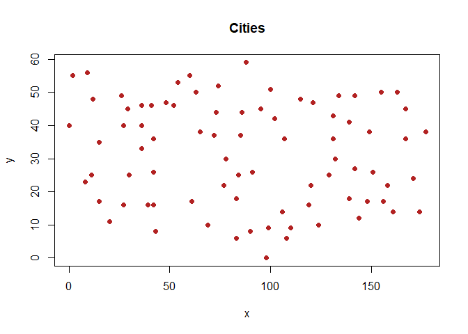
Plotting the Raw Data
1
2
plot(data[c("x","y")], main = "Cities",
     xlab = "x", ylab = "y", pch = 19, col = "firebrick")
Figure 1. Coordinates of the Cities
Algorithm: SOM-TSP
1
2
3
4
5
6
7
8
9
10
11
12
13
14
15
16
17
18
19
20
21
22
23
24
25
26
27
28
29
30
31
32
33
34
35
36
37
38
39
40
41
42
43
44
45
46
47
48
49
50
51
som_tsp <- function(X, I = 81, nf, alpha = 0.9, beta = 0.9, sigma, eta = 0.9, iter){
    # X -> Coordinates and names of  the cities (an n by 3 data frame)
    n <- nrow(X)
    # I -> Number of neurons
    # nf -> Neighborhood function
    # iter -> number of iterations

    t <- 0 # Set counter t=0
    # Locate I neurons randomly
    # (Create an I by 2 matrix whose x and y's are randomly picked from the uniform
    # distribution between the minimum and maximum values of the city coordinates)

    w <- cbind(matrix(runif(I, min(X[ ,"x"]), max(X[ ,"x"])),
                      nrow = I),
               matrix(runif(I, min(X[ ,"y"]), max(X[ ,"y"])),
                      nrow = I)                                 )

    repeat{
        # Put cities in random order
        X <- X[sample(1:n), ]

        # Determine the winning neuron and "neighborhood"
        for (p in 1:n){
            # Get the index of the minimum Euclidean norm of x_p - w_i
            ip <- which.min(mapply(enorm,
                                   sweep(w, 2, as.numeric(X[p, -1]))[ ,1],
                                   sweep(w, 2, as.numeric(X[p, -1]))[ ,2]   )   )

            for (i in 1:I){
                # Apply neighborhood function
                neighborhood <- nf(I, w, sigma, ip, i)
                w[i, ] <- as.numeric(w[i, ] + alpha*neighborhood*(X[p, -1] - w[i, ]))
            } # end for
        } # end for

        # Update parameters
        sigma <- beta*sigma
        alpha <- eta*alpha
        t <- t + 1

        # Stopping condition (Reaching the desired number of iterations)
        if(t == iter){
            break
        }
    }

    # Return an (n+I) by 3 matrix which includes cities and neurons
    neurons <- cbind(c(1:I), w)
    colnames(neurons) <- c("city", "x", "y")
    return(rbind(X, neurons))
}
Running the Algorithm
1
2
3
4
5
6
7
8
9
10
11
12
13
14
15
16
17
18
19
20
21
22
23
24
25
26
27
28
29
30
31
32
33
34
35
36
37
38
39
40
41
42
43
44
45
46
47
48
49
50
51
52
53
54
55
56
57
58
59
60
61
62
63
64
65
66
67
68
69
70
71
72
73
74
75
# Standard deviation of all city coordinates can be used as an initial value for sigma
s <- sd(c(data[ , "x"], data[ , "y"]))

# Alpha, beta, and eta will be left as default, all of which are 0.9
# Running the algorithm with 100 iterations:

# A) with Gaussian Kernel and M = n

gk_n <- som_tsp(data, I = 81, gaussian_kernel,
                sigma = s, iter = 100)

results_gk_n <- results(data, gk_n)

dist_gk_n <- ttd(results_gk_n)

# B) with Gaussian Kernel and M = 2n

gk_2n <- som_tsp(data, I = 162, gaussian_kernel,
                sigma = s, iter = 100)

results_gk_2n <- results(data, gk_2n)

dist_gk_2n <- ttd(results_gk_2n)

# C) with Gaussian Kernel and M = 3n

gk_3n <- som_tsp(data, I = 243, gaussian_kernel,
                sigma = s, iter = 100)

results_gk_3n <- results(data, gk_3n)

dist_gk_3n <- ttd(results_gk_3n)

# D) with Elastic Band and M = n

eb_n <- som_tsp(data, I = 81, elastic_band,
                sigma = s, iter = 100)

results_eb_n <- results(data, eb_n)

dist_eb_n <- ttd(results_eb_n)

# E) with Elastic Band and M = 2n

eb_2n <- som_tsp(data, I = 162, elastic_band,
                sigma = s, iter = 100)

results_eb_2n <- results(data, eb_2n)

dist_eb_2n <- ttd(results_eb_2n)

# F) with Elastic Band and M = 3n

eb_3n <- som_tsp(data, I = 243, elastic_band,
                sigma = s, iter = 100)

results_eb_3n <- results(data, eb_3n)

dist_eb_3n <- ttd(results_eb_3n)

# Extra trials for M = 2n and 1000 iterations

# Gaussian Kernel
gk_2n_1k <- som_tsp(data, I = 162, gaussian_kernel, sigma = s, iter = 1000)

results_gk_2n_1k <- results(data, gk_2n_1k)

dist_gk_2n_1k <- ttd(results_gk_2n_1k)

# Elastic Band
eb_2n_1k <- som_tsp(data, I = 162, elastic_band, sigma = s, iter = 1000)

results_eb_2n_1k <- results(data, eb_2n_1k)

dist_eb_2n_1k <- ttd(results_eb_2n_1k)
Results
Suggested travel plans with objective values and first/last stops:
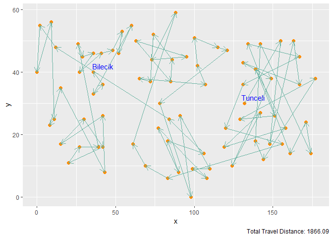
Figure 2. Gaussian Kernel with M = n Neurons and 100 Iterations
Figure 3. Gaussian Kernel with M = 2n Neurons and 100 Iterations
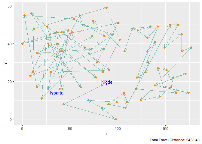
Figure 4. Gaussian Kernel with M = 3n Neurons and 100 Iterations
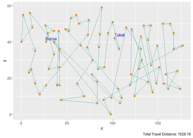
Figure 5. Gaussian Kernel with M = 2n Neurons and 1000 Iterations
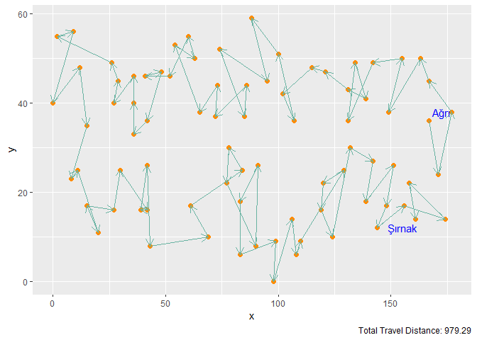
Figure 6. Elastic Band with M = n Neurons and 100 Iterations
Figure 7. Elastic Band with M = 2n Neurons and 100 Iterations
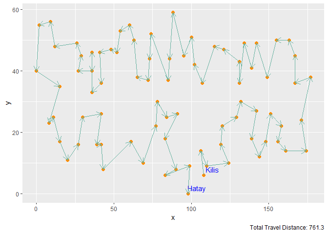
Figure 8. Elastic Band with M = 3n Neurons and 100 Iterations
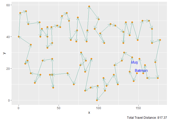
Figure 9. Elastic Band with M = 2n Neurons and 1000 Iterations
Summary of the Results
1
2
3
4
5
6
7
8
9
10
11
12
13
14
n_function  <- c(rep("Gaussian Kernel", 4), rep("Elastic Band", 4))
neurons     <- rep(c("n", "2n", "3n", "2n"), 2)
iterations  <- rep(c(100, 100, 100, 1000), 2)
distance    <- c(ttd(results_gk_n), ttd(results_gk_2n), ttd(results_gk_3n),
                 ttd(results_gk_2n_1k),
                 ttd(results_eb_n), ttd(results_eb_2n), ttd(results_eb_3n),
                 ttd(results_eb_2n_1k))

summary <- data.frame(matrix(c(n_function, neurons, iterations, distance), ncol = 4))

colnames(summary) <- c("Neigborhood Function", "Number of Neurons",
                       "Number of Iterations", "Total Travel Distance")

knitr::kable(summary, "simple", row.names = FALSE)
| Neigborhood Function | Number of Neurons | Number of Iterations | Total Travel Distance |
|---|---|---|---|
| Gaussian Kernel | n | 100 | 1702.39 |
| Gaussian Kernel | 2n | 100 | 1866.09 |
| Gaussian Kernel | 3n | 100 | 2438.48 |
| Gaussian Kernel | 2n | 1000 | 1528.19 |
| Elastic Band | n | 100 | 979.29 |
| Elastic Band | 2n | 100 | 806.21 |
| Elastic Band | 3n | 100 | 761.3 |
| Elastic Band | 2n | 1000 | 817.37 |
Final Comments
According to the final summary table, Gaussian Kernel works better with higher number of iterations since the 1000 iterations trial have yielded the shortest route. When the divergence in the first three trials are considered, increasing the number of neurons had a negative effect for this neighborhood function.
In contrast, for the Elastic Band function, 3n neurons have yielded the best travel plan, which is also the best obtained result among all trials.
Due to the significant difference between their best distances (Elastic Band’s best solution suggests a 2 times shorter path), it can be concluded that in the specific case of Traveling Salesman Problem, SOM works better with the neighborhood function defined on the elastic band.
IE 440 - Nonlinear Models in Operations Research
Boğaziçi University - Industrial Engineering Department
GitHub Repository
