Leukemia describes a group of blood disorders characterized by the dysfunctional production and development of lymphocytes, a type of white blood cell.
In this notebook, 2 different models are provided to solve multiclass classification problem on leukemia gene expression dataset from Curated Microarray Database (CuMiDa).
The common challenge in gene expression arrays is that they violate the assumption that the number of samples is higher than the number of predictors (p » n). Therefore, Naive Bayes Classifier and Support Vector Machines will be used as model algorithms, which perform well on such data most of the time. The dimensionality of the original dataset will be reduced by decomposing it into principal components and keeping the principal components that explain the 90% of the variance. The reduced version of the data will be feeding the Support Vector Classifier.
Libraries
1
2
3
4
5
6
7
8
9
10
11
12
13
14
15
| import numpy as np
import pandas as pd
import matplotlib.pyplot as plt
%matplotlib inline
import seaborn as sns
from sklearn.model_selection import train_test_split
from sklearn.model_selection import GridSearchCV, cross_val_score
from sklearn.decomposition import PCA
from sklearn.metrics import accuracy_score, confusion_matrix
from sklearn.naive_bayes import GaussianNB
from sklearn.svm import SVC
|
Importing and Preprocessing the Data
1
| data = pd.read_csv('./Data/Leukemia_GSE9476.csv')
|
1
2
| print(data.shape)
data.head()
|
| samples | type | 1007_s_at | 1053_at | 117_at | 121_at | 1255_g_at | 1294_at | 1316_at | 1320_at | ... | AFFX-r2-Hs28SrRNA-5_at | AFFX-r2-Hs28SrRNA-M_at | AFFX-r2-P1-cre-3_at | AFFX-r2-P1-cre-5_at | AFFX-ThrX-3_at | AFFX-ThrX-5_at | AFFX-ThrX-M_at | AFFX-TrpnX-3_at | AFFX-TrpnX-5_at | AFFX-TrpnX-M_at |
|---|
| 0 | 1 | Bone_Marrow_CD34 | 7.745245 | 7.811210 | 6.477916 | 8.841506 | 4.546941 | 7.957714 | 5.344999 | 4.673364 | ... | 5.058849 | 6.810004 | 12.800060 | 12.718612 | 5.391512 | 4.666166 | 3.974759 | 3.656693 | 4.160622 | 4.139249 |
|---|
| 1 | 12 | Bone_Marrow_CD34 | 8.087252 | 7.240673 | 8.584648 | 8.983571 | 4.548934 | 8.011652 | 5.579647 | 4.828184 | ... | 4.436153 | 6.751471 | 12.472706 | 12.333593 | 5.379738 | 4.656786 | 4.188348 | 3.792535 | 4.204414 | 4.122700 |
|---|
| 2 | 13 | Bone_Marrow_CD34 | 7.792056 | 7.549368 | 11.053504 | 8.909703 | 4.549328 | 8.237099 | 5.406489 | 4.615572 | ... | 4.392061 | 6.086295 | 12.637384 | 12.499038 | 5.316604 | 4.600566 | 3.845561 | 3.635715 | 4.174199 | 4.067152 |
|---|
| 3 | 14 | Bone_Marrow_CD34 | 7.767265 | 7.094460 | 11.816433 | 8.994654 | 4.697018 | 8.283412 | 5.582195 | 4.903684 | ... | 4.633334 | 6.375991 | 12.903630 | 12.871454 | 5.179951 | 4.641952 | 3.991634 | 3.704587 | 4.149938 | 3.910150 |
|---|
| 4 | 15 | Bone_Marrow_CD34 | 8.010117 | 7.405281 | 6.656049 | 9.050682 | 4.514986 | 8.377046 | 5.493713 | 4.860754 | ... | 5.305192 | 6.700453 | 12.949352 | 12.782515 | 5.341689 | 4.560315 | 3.887020 | 3.629853 | 4.127513 | 4.004316 |
|---|
5 rows × 22285 columns
1
| data['type'].value_counts()
|
1
2
3
4
5
6
| AML 26
Bone_Marrow 10
PB 10
PBSC_CD34 10
Bone_Marrow_CD34 8
Name: type, dtype: int64
|
1
2
3
4
| # Replacing labels with numeric values
data["type"] = data["type"].replace({"AML":0, "Bone_Marrow":1, "PB":2, "PBSC_CD34":3, "Bone_Marrow_CD34":4})
# Storing label names in a list
labels = ["AML", "Bone_Marrow", "PB", "PBSC_CD34", "Bone_Marrow_CD34"]
|
Train-Test Split
1
2
3
4
5
| X = data.drop(["type"], axis=1)
y = data["type"]
# using the train test split function
X_train, X_test, y_train, y_test = train_test_split(X, y, random_state=200, test_size=0.30, shuffle=True)
|
Principal Component Analysis
1
2
| pca = PCA()
pca.fit_transform(X_train)
|
1
2
3
4
5
6
7
8
9
10
11
12
13
| array([[ 7.42136611e+01, -2.18219666e+01, -1.70596309e+01, ...,
1.69833896e+00, 1.65937536e+00, 1.27173212e-13],
[ 2.20025774e+01, 4.37665430e+01, -1.27529875e+01, ...,
8.35724135e-02, -9.58648421e-01, 1.27173212e-13],
[-8.31658114e+00, -2.42812693e+01, -2.09776274e+01, ...,
-3.89558842e-01, -8.52854616e-03, 1.27173212e-13],
...,
[ 2.36180585e+01, 3.74960783e+01, -2.36891534e+01, ...,
-4.22934933e+00, 1.24303529e+01, 1.27173212e-13],
[-1.60907152e+01, -1.68696788e+01, 1.83121977e+01, ...,
2.19669798e-01, -1.57023579e-01, 1.27173212e-13],
[ 4.35651139e+01, 1.13885969e+01, 5.10196868e+01, ...,
-7.98296444e-02, 2.49958631e-01, 1.27173212e-13]])
|
1
2
3
4
5
6
7
8
9
10
11
12
13
14
15
16
17
18
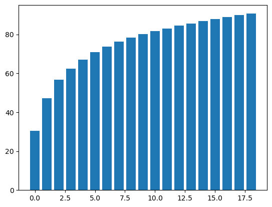
| total = sum(pca.explained_variance_)
k = 0
current_variance = 0
while current_variance/total < 0.90:
current_variance += pca.explained_variance_[k]
k = k + 1
print(k, " features explain around 90% of the variance.", sep='')
pca = PCA(n_components=k)
X_train.pca = pca.fit(X_train)
X_train_pca = pca.transform(X_train)
X_test_pca = pca.transform(X_test)
var_exp = pca.explained_variance_ratio_.cumsum()
var_exp = var_exp*100
plt.bar(range(k), var_exp);
|
1
| 19 features explain around 90% of the variance.
|
Figure 1. Cumulative % Explained Variance Sums
1
2
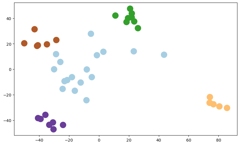
| pca_2 = PCA(n_components=2).fit(X_train)
X_train_reduced = pca_2.transform(X_train)
|
1
2
| fig = plt.figure(1, figsize = (10, 6))
plt.scatter(X_train_reduced[:, 0], X_train_reduced[:, 1], c = y_train, cmap = plt.cm.Paired, linewidths=10)
|
1
| <matplotlib.collections.PathCollection at 0x1ebb669ba00>
|
Figure 2. Plot of the 2D Reduced Version
Clusters can be seen clearly when the data is reduced to 2D.
Modeling
Baseline
Firstly, the accuracy score of simply predicting each test observation as the dominating class, which is acute myeloid leukemia (AML) in this case, can be checked as a baseline.
1
2
| base_acc = len(y_test[y_test == 0])/len(y_test)*100
print("Baseline Accuracy ", round(base_acc, 3), "%", sep = '')
|
1
| Baseline Accuracy 45.0%
|
Naive Bayes Classifier
1
2
3
4
5
6
7
8
9
10
11
12
13
14
15
16
17
18
19
20
21
22
23
| # Model
nb_model = GaussianNB()
nb_model.fit(X_train, y_train)
# Prediction
nb_pred = nb_model.predict(X_test)
# Accuracy
nb_acc = accuracy_score(y_test, nb_pred)*100
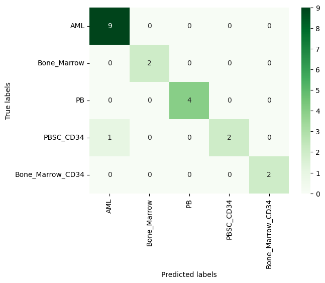
print('Naive Bayes Accuracy: ', round(nb_acc, 3), "%", sep="")
# Confusion Matrix
cm_nb = confusion_matrix(y_test, nb_pred)
# Plot
ax = plt.subplot()
sns.heatmap(cm_nb, annot=True, ax=ax, fmt='g', cmap='Greens')
# labels, title and ticks
ax.set_xlabel('Predicted labels')
ax.set_ylabel('True labels')
ax.xaxis.set_ticklabels(labels, rotation=90)
ax.yaxis.set_ticklabels(labels, rotation=360);
|
1
| Naive Bayes Accuracy: 95.0%
|
Figure 3. Confusion Matrix of Naive Bayes
Support Vector Machines
1
2
3
4
5
6
7
8
9
10
11
12
13
14
15
16
17
18
19
20
21
22
23
24
25
26
27
28
29
30
31
32
33
34
| # Parameter grid
svm_param_grid = { 'C': [0.1, 1, 10, 100],
"decision_function_shape" : ["ovo", "ovr"],
'gamma': [1, 0.1, 0.01, 0.001, 0.00001, 10],
"kernel": ["linear", "rbf", "poly"]}
# Creating the SVM grid search classifier
svm_grid = GridSearchCV(SVC(), svm_param_grid, cv=3)
# Training the classifier
svm_grid.fit(X_train_pca, y_train)
print("Best Parameters:\n", svm_grid.best_params_)
# Selecting the best SVC
best_svc = svm_grid.best_estimator_
# Predictions
svm_pred = best_svc.predict(X_test_pca)
# Accuracy
svc_acc = accuracy_score(y_test, svm_pred)*100
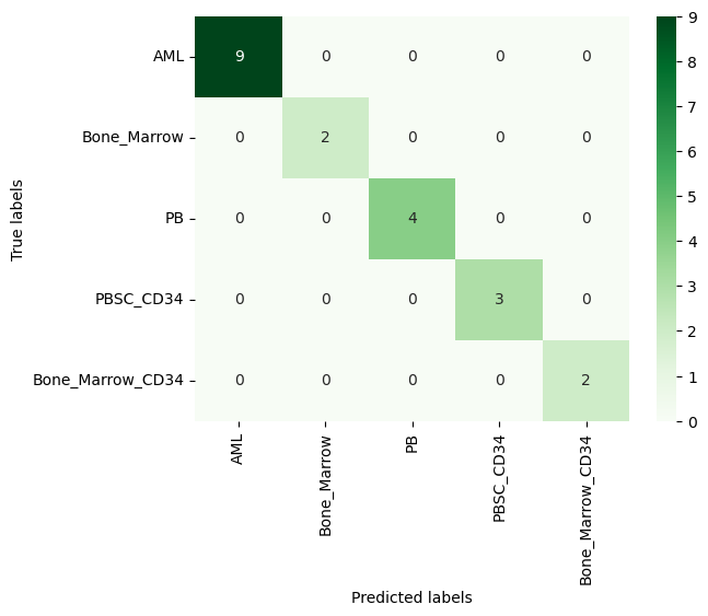
print('SVM Accuracy: ', round(svc_acc, 3), "%", sep="")
cm_svm = confusion_matrix(y_test, svm_pred)
ax = plt.subplot()
sns.heatmap(cm_svm, annot=True, ax = ax, fmt='g', cmap='Greens')
# Labels, title and ticks
ax.set_xlabel('Predicted labels')
ax.set_ylabel('True labels')
ax.xaxis.set_ticklabels(labels, rotation=90)
ax.yaxis.set_ticklabels(labels, rotation=360);
|
1
2
3
| Best Parameters:
{'C': 10, 'decision_function_shape': 'ovo', 'gamma': 1e-05, 'kernel': 'rbf'}
SVM Accuracy: 100.0%
|
Figure 4. Confusion Matrix of Support Vector Classifier
As can be seen from the confusion matrices, both models perform well. If a larger part of the dataset (i.e. 75%) were used as training data, Naive Bayes would also reach to perfect classification.
Note that the models might not perform as well as this case on different datasets or might require further configurations, since the dataset used in this notebook is extremely clean.
Inspired by Gene Expression Classification
GitHub Repository