Introduction
In this short example, the aim is to predict Toyota Corolla prices by taking the fields such as age, kilometers, fuel type etc. into consideration. The tree will be pruned according to the cross-validation error.
Importing the Data and the Required Libraries
1
2
3
4
5
6
7
8
9
10
11
12
13
14
15
16
17
18
19
20
21
22
23
24
|
library(rpart)
library(rpart.plot)
library(caret)
library(tree)
library(caTools)
library(dplyr)
library(Metrics)
tc <- read.csv("ToyotaCorolla.csv")
seed <- 425
set.seed(seed)
# Partitioning the data set into training and test sets
split <- sample.split(tc$Price, SplitRatio = 0.80)
tctrain <- subset(tc, split == TRUE)
tctest <- subset(tc, split == FALSE)
nrow(tctrain)
|
Generating and Pruning the Tree
1
2
3
4
5
6
7
8
|
tree <- rpart(Price~., data = tctrain)
prp(tree,
type = 5,
extra = 1,
tweak = 1)
|
Figure 1. Decision tree before pruning
1
| cpTable <- printcp(tree)
|
1
2
3
4
5
6
7
8
9
10
11
12
13
14
15
16
17
18
19
20
| ##
## Regression tree:
## rpart(formula = Price ~ ., data = tctrain)
##
## Variables actually used in tree construction:
## [1] Age KM Weight
##
## Root node error: 1.62e+10/1177 = 13763705
##
## n= 1177
##
## CP nsplit rel error xerror xstd
## 1 0.665025 0 1.00000 1.00249 0.070271
## 2 0.105496 1 0.33497 0.33830 0.022141
## 3 0.037143 2 0.22948 0.23329 0.021563
## 4 0.019794 3 0.19234 0.20448 0.012577
## 5 0.015178 4 0.17254 0.18820 0.012629
## 6 0.015150 5 0.15736 0.17962 0.012932
## 7 0.010251 6 0.14221 0.16113 0.011785
## 8 0.010000 7 0.13196 0.15558 0.011671
|
1
2
3
4
5
6
7
8
|
# Reporting the number of terminal nodes in the tree with the lowest cv-error,
# which is equal to [the number of splits performed to create the tree] + 1
optIndex <- which.min(unname(tree$cptable[, "xerror"]))
cpTable[optIndex, 2] + 1
|
The generated tree has 8 terminal nodes.
1
2
3
4
5
6
7
|
# Pruning the tree to the optimized cp value
optTree <- prune.rpart(tree = tree, cp = cpTable[optIndex, 1])
prp(optTree)
|
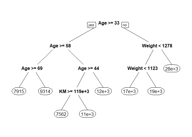
Figure 2. Decision tree after pruning
1
2
3
4
5
6
7
8
9
|
# Making predictions in the test set
pred <- predict(optTree, newdata = tctest)
# Reporting the metrics
# Root mean squared error
rmse(actual = tctest$Price, predicted = pred)
|
1
2
3
| # Mean absolute error
mae (actual = tctest$Price, predicted = pred)
|
IE 425 - Data Mining
Boğaziçi University - Industrial Engineering Department
GitHub Repository