Introduction
In this exercise, predictions on the financial conditions of the companies given in the data set Financialdistress-cat.csv will be held. The output attribute to be predicted is the Financial.Distress attribute, which is zero if the company is in a healthy condition, one otherwise.
One can check the GitHub repository for further details.
The first step is importing the required libraries and the data set.
1
2
3
4
5
6
7
8
9
10
11
12
13
14
15
16
17
18
19
20
21
22
23
24
25
26
27
28
library(rpart)
library(rpart.plot)
library(caret)
library(tree)
library(caTools)
library(dplyr)
library(Metrics)

fd <- read.csv("FinancialDistress-cat.csv")
fd$Financial.Distress <- as.factor(fd$Financial.Distress)

# Splitting the data set into training and test

set.seed(425)

split1  <- sample.split(fd$Financial.Distress, SplitRatio = 0.75)

fdtrain <- subset(fd, split1==TRUE)
fdtest  <- subset(fd, split1==FALSE)

prcntfd   <- nrow(dplyr::filter(fd,      Financial.Distress %in% 1)) / nrow(fd)
prcnttr   <- nrow(dplyr::filter(fdtrain, Financial.Distress %in% 1)) / nrow(fdtrain)
prcnttest <- nrow(dplyr::filter(fdtest,  Financial.Distress %in% 1)) / nrow(fdtest)

percentages        <- 100*c(prcntfd  , prcnttr   , prcnttest )
names(percentages) <-     c("overall", "training", "test"    )

knitr::kable(round(percentages, 3), "simple", col.names = "Distress %")
| Distress % | |
|---|---|
| overall | 6.863 |
| training | 6.863 |
| test | 6.863 |
Table 1. Percentage of companies in distress in the original and split data sets
The percentages look pretty much the same, which implies that the data set is suitable for a homogeneous split with high precision.
Generating and Pruning the Tree (Based on the Cross-Validation Error)
The next step is to determine the best size of the best tree in terms of cross validation error.
1
2
3
4
5
6
7
8
9
10
11
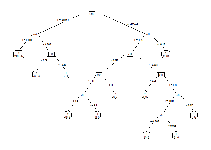
# Generating the tree (Parameters are chosen intuitively and also by trial and error.)

treeA <- rpart(Financial.Distress~.,
               data      = fdtrain,
               minsplit  = 30,
               minbucket = 8)

prp(treeA,
    type    = 5,
    extra   = 1,
    tweak   = 1)
Figure 1. Decision tree before pruning
Checking the CP table:
1
2
cpTable <- printcp(treeA)
knitr::kable(cpTable, "simple", row.names = FALSE)
| CP | nsplit | rel error | xerror | xstd |
|---|---|---|---|---|
| 0.1216931 | 0 | 1.0000000 | 1.0000000 | 0.0701990 |
| 0.1005291 | 1 | 0.8783069 | 1.0529101 | 0.0718916 |
| 0.0476190 | 2 | 0.7777778 | 0.8571429 | 0.0653328 |
| 0.0423280 | 3 | 0.7301587 | 0.8888889 | 0.0664546 |
| 0.0185185 | 4 | 0.6878307 | 0.8306878 | 0.0643787 |
| 0.0158730 | 6 | 0.6507937 | 0.8783069 | 0.0660834 |
| 0.0132275 | 7 | 0.6349206 | 0.9100529 | 0.0671891 |
| 0.0105820 | 9 | 0.6084656 | 0.9259259 | 0.0677331 |
| 0.0100000 | 10 | 0.5978836 | 0.9523810 | 0.0686273 |
Table 2. CP Table
Pruning the tree:
1
2
3
4
5
6
# Reporting the number of terminal nodes in the tree with the lowest cv-error,
# which is equal to [the number of splits performed to create the tree] + 1

optIndex <- which.min(unname(treeA$cptable[, "xerror"]))

cpTable[optIndex, 2] + 1
1
## [1] 5
1
2
3
4
5
6
# Pruning the tree to the optimized cp value

optTree <- prune.rpart(tree = treeA,
                       cp   = cpTable[optIndex, 1])

prp(optTree)
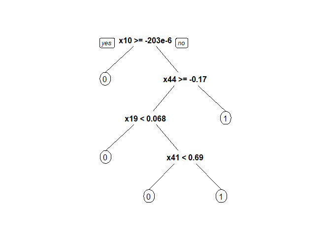
Figure 2. Decision tree after pruning
As the cp table generated by the R script suggests, the tree with 2 splits and 3 terminal nodes yields the lowest cross-validation error.
Predictions (Minimizing CV Error)
Predictions can be made in the test set along with reporting the error rate, sensitivity, specificity, and precision using the confusionMatrix function of the caret package.
1
2
3
4
5
6
7
8
9
10
# Making predictions in the test set and tabulating the results

predA    <- predict(optTree,
                    newdata = fdtest,
                    type = "class")

tblA     <- table(fdtest$Financial.Distress,
                  predA)

knitr::kable(tblA, "simple", col.names = c("pred_0", "pred_1"))
| pred_0 | pred_1 | |
|---|---|---|
| 0 | 842 | 13 |
| 1 | 37 | 26 |
Table 3. Prediction results
1
2
3
4
5
6
7
8
9
10
11
12
13
14
# Generating the confusion matrix

cmA <- confusionMatrix(predA, fdtest$Financial.Distress, positive = "1")

# Reporting the metrics

results <- matrix(c(cmA[["overall"]][["Accuracy"]]   ,
                    cmA[["byClass"]][["Sensitivity"]],
                    cmA[["byClass"]][["Specificity"]],
                    cmA[["byClass"]][["Precision"]]  ), ncol = 1)

rownames(results) <- c('Accuracy', 'Sensitivity', "Specificity", "Precision")

knitr::kable(round(results, 3)*100, "simple", col.names = "%")
| % | |
|---|---|
| Accuracy | 94.6 |
| Sensitivity | 41.3 |
| Specificity | 98.5 |
| Precision | 66.7 |
Table 4. Prediction report
Pruning the Tree (Based on the Cost Complexity)
The raw tree can be alternatively pruned by minimizing the cost complexity, which is measured by the deviance in the tree package.
To obtain the tree with the smallest deviance, the minsize and mindev parameters should be set to the minimum values they can take, 2 and 0, in the tree function.
1
2
3
4
5
6
7
8
9
10
# Creating a tree with terminal nodes that all have zero deviance

treeB <- tree(Financial.Distress~.,
              data      = fdtrain,
              minsize   = 2,
              mindev    = 0.0)

# Reporting the number of terminal nodes

summary(treeB)[["size"]]
1
## [1] 89
Predictions (Minimizing Cost Complexity)
1
2
3
4
5
6
7
8
9
# Making predictions in the test set and tabulating the results

predB   <- predict(treeB,
                   newdata = fdtest,
                   type = "class")

tblB    <- table(fdtest$Financial.Distress, predB)

knitr::kable(tblB, "simple", col.names = c("pred_0", "pred_1"))
| pred_0 | pred_1 | |
|---|---|---|
| 0 | 823 | 24 |
| 1 | 39 | 24 |
Table 5. Prediction results (alternative pruning)
1
2
3
4
5
6
7
8
9
10
11
12
# Generating the confusion matrix

cmB <- confusionMatrix(predB, fdtest$Financial.Distress, positive = "1")

# Reporting the metrics and comparison with part C

results <- cbind(results, c(cmB[["overall"]][["Accuracy"]],
                            cmB[["byClass"]][["Sensitivity"]],
                            cmB[["byClass"]][["Specificity"]],
                            cmB[["byClass"]][["Precision"]]   ))

knitr::kable(round(results, 3), "simple", col.names = c("Cross-Validation", "Cost Complexity"))
| Cross-Validation | Cost Complexity | |
|---|---|---|
| Accuracy | 0.946 | 0.923 |
| Sensitivity | 0.413 | 0.381 |
| Specificity | 0.985 | 0.963 |
| Precision | 0.667 | 0.429 |
Table 6. Performance comparison of the two models
As can be expected, the tree pruned by minimizing the cross-validation error has better accuracy, specificity, and precision compared to the one pruned according to cost complexity, which has lost some of its general validity due to its perfect fit. In other words, too many terminal nodes might lead the model to overfitting!
IE 425 - Data Mining
Boğaziçi University - Industrial Engineering Department
GitHub Repository


